The low-pass filter frequency response

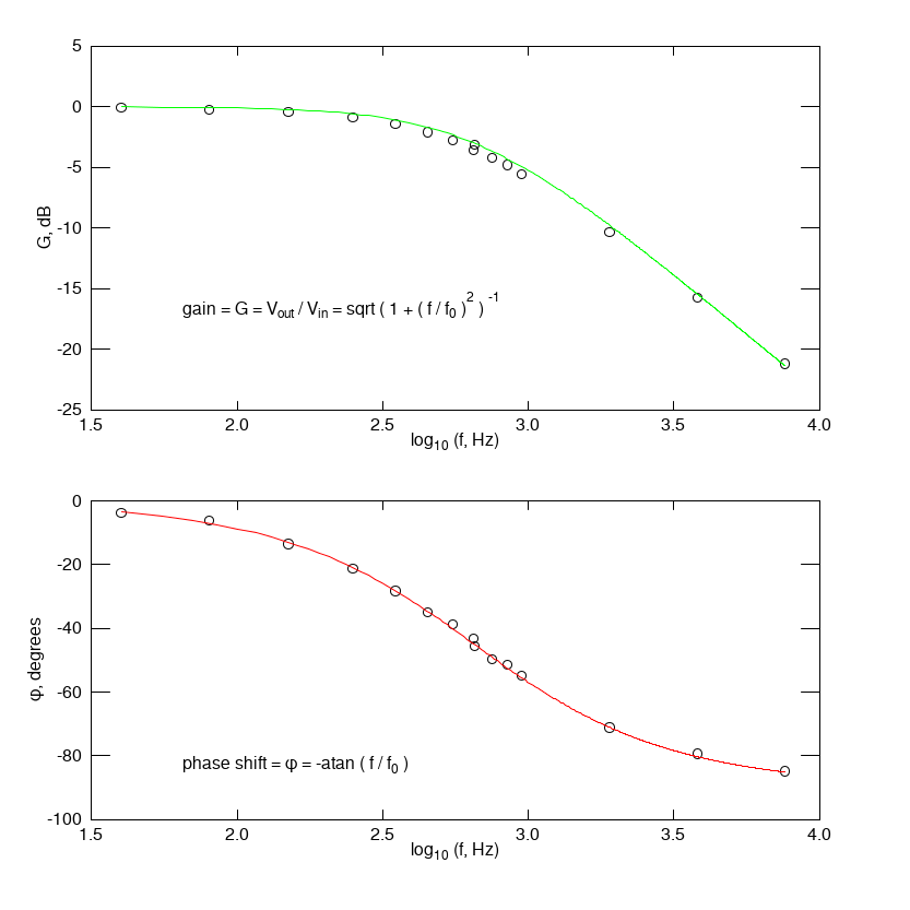
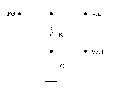
A low pass filter attenuates the amplitude of frequencies above the filter centre frequency f₀ while leaving those below f₀ unchanged. A sine wave of amplitude V_in and frequency f input to the filter will output a sine wave with amplitude V_out and the same f but phase shifted to some extent from the input signal .

Shown are typical gain G and phase shift φ plots rendered using eXtrema. The centre frequency of a low-pass filter is

f₀ = 1/(2πRC).

The filter gain G(f) is the ratio of input and output amplitudes

G(f) = V_out(f)/V_in(f) = 1 / (sqrt ( 1 + ( f / f₀ )² ))

and the phase shift of the output signal relative to the input is

φ(f) = -atan ( f / f₀ )

Shown is the schematic diagram of the RC low pass filter used to generate the plots in the previous slide. Begin by assembling the circuit shown with measured values of C~0.01μF and R~10kΩ, then connect V_in to the scope CH1 input and V_out to CH2.

Calculate the theoretical F₀ for this filter, then make a table of n well chosen test frequencies f_n that will be used to plot G(f) and φ(f). For each of these frequencies:

• verify that CH1, CH2 Voltage is set to 1X;
• measure and tabulate V_in(f_n), V_out(f_n);
• measure the time delay Δt_n between V_in(f_n) and V_out(f_n);
• calculate and tabulate G(f_n), T_n, φ(f_n).

Plot log G(f) vs. log(f) and φ(f) vs. log(f). From the graphs, identify and estimate the gain and φ at f₀ and the filter roll-off rate in dB/octave. Add more f_n points to the graphs, if necessary.

• What are the theoretical values for G(f₀) and φ(f₀)?
• Compare these with the results from the graphs.

Gain and φ plots of a low-pass filter

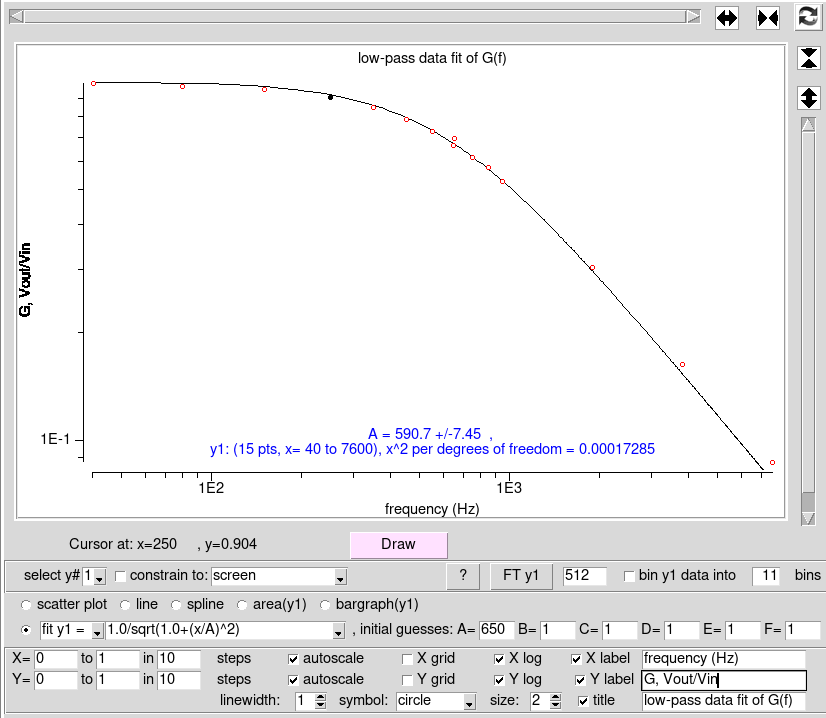
You can also determine some values for f₀ by fitting the G(f) and φ(f) equations to your data sets as shown in the first slide. To perform these fits, use eXtrema or any other software.

PhysTks, shown here, is a simple to use plotting and fitting app. Type PhysTks in a terminal window, then enter your data and click Draw to plot the data set. You do not need to calculate log(G) and log(f), simply check the Xlog and Ylog boxes.

To fit the G(f) equation enter: 1.0/sqrt(1.0+(x/A)^2) and set the fit parameter A to the calculated f₀ as an initial guess. Check Fit, click Draw; the new A value displayed is the f₀ result from the fit. Check also that the rolloff is as expected.

For the φ fit, set A as before, then enter -atan(x/A)*180/$pi since the atan result will be in radians.

• Compare these fitted f₀ results with the calculated f₀.

The Lissajous curve

Assuming that CH1 (V_x) monitors V_in(f) and CH2 (V_y) monitors V_out(f), then the gain and the phase shift are given by:

G(f) = b / a    and     φ(f) = arcsin ( c / b )

To center the ellipse on the scope screen, click the menu button in the HORIZONTAL scope settings, then:

• select CH1, click Coupling button unitl appears;
• place the resulting vertical line over the y-axis;
• click Coupling button until appears;
• repeat for CH2 to place the horizontal line over the x-axis.

Set the FG frequency to f0 and measure a, b and c, then compare G(f0) and φ(f0) with your previous results.