Exploring the timing of the mystery circuit
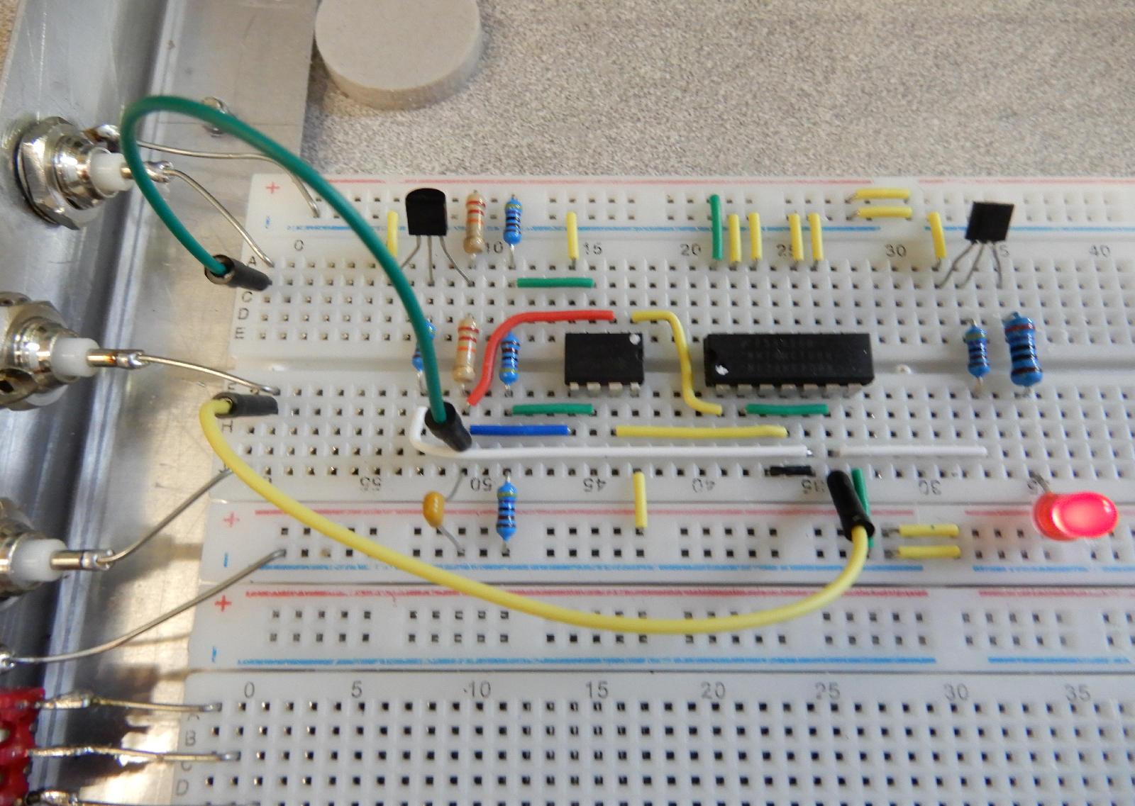
- Connect a BNC (Bayonet Neill–Concelman) coaxial cable from scope CH2 to a workstation BNC jack, then use a jumper to connect the jack to pin 6 of IC2.
- Press the
Autosetbutton. A blue CH2 trace should appear. - Rotate the TIME/DIV knob until the time/div display reads '100ms ROLL'.
- Set the CH2 VOLTS/DIV to 1V, then rotate the CH2 up/down position knob to display a square wave moving across the screen. What does this waveform represent?
- Replace C with a 0.1μF capacitor, then press
Autoset. What is the time/div now? - The LED appears always on. Why might this be so?
- How does the choice of capacitor (i.e. capacitance) affect the timing mystery circuit?
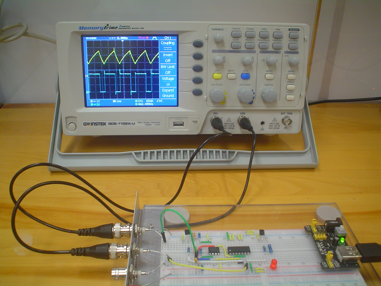
You can now use the oscilloscope to explore the mystery circuit. Save screenshots of each test then make a sketch showing how the various waveforms are related in time.
- Connect a second BNC cable from the scope CH1 to a workstation BNC jack, then use a jumper to connect the jack to the R5-C node.
- Press the
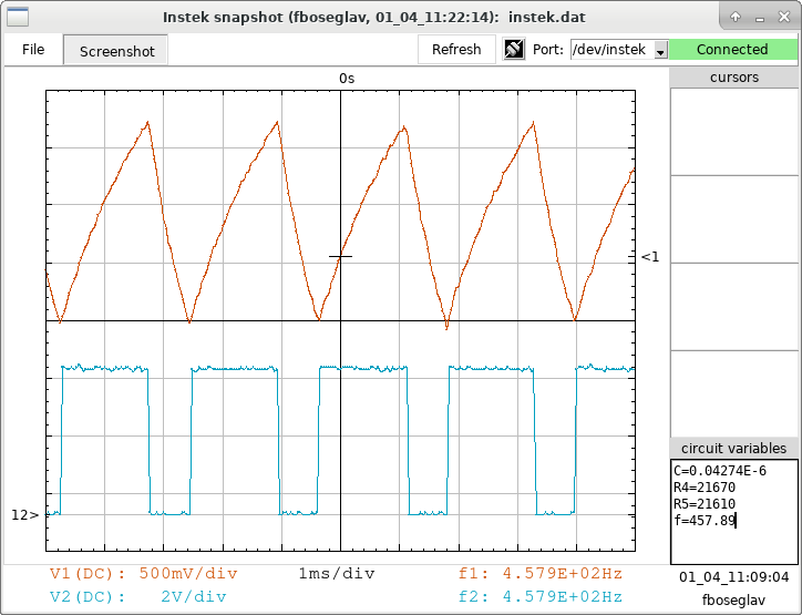
Autosetbutton. Two waveform should appear, as in the previous slide. The yellow CH1 waveform displays the variation in the capacitor voltage Vc. How do the two waveforms compare? - How are the waveforms at pin 1 and 7 of IC1 related to Vc?
- How are the waveforms at pin 5 and 6 of IC2 related to Vc?
- What does pin 5 of IC2 control? and pin 6 of IC2?
You can now proceed to measure TL, TH and T as you vary R4, R5 or C and populate a table with the results. You can then determine the scaling constants k1 and k2.
- Use the Component Tester (CT) to measure the capacitors.
- Re-measure the resistors more precisely with the multimeter and compare with the previous CT results.
- In a terminal window, type GDS-1102A to invoke the app that connects to the scope and streams the scope output to the computer screen.
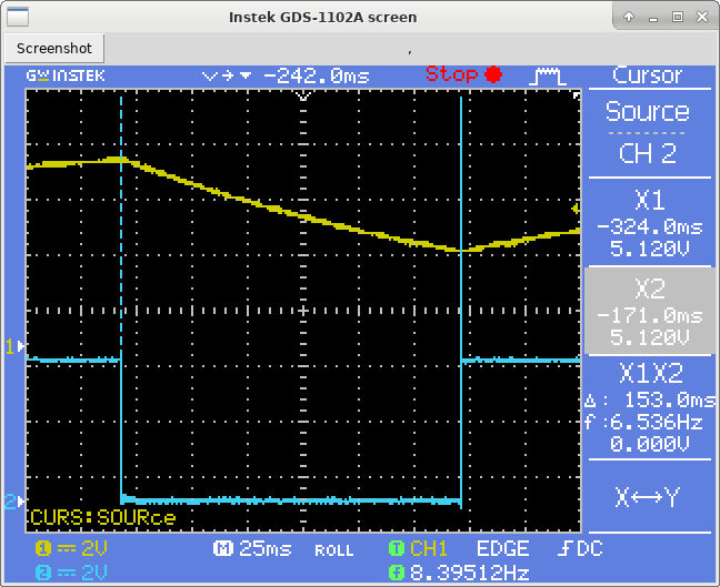
- With Ch1 connected to the R5-C node and Ch2 connected to IC2 pin 6, press
the
Autosetbutton to view the two waveforms, as shown.
We note that the observed pulse waveform seem to repeat with a period T that consists of a low level time TL and a high level time TH, so that T=TL+TH.
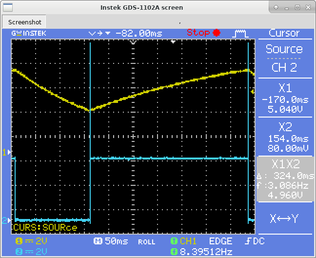
Note that since the transitions of the two waveforms seem to occur at the same time, you can place the cursors more accurately using the square wave as reference.
For each measurement of TL, or TH as shown, check that the cursors and the cursor data are displayed and that the correct values of R4, R5, C are entered in the variables frame.
Save the data set (click 'File', 'Save data') and a screenshot of every trial. From a Linux workstation, save distinctly labelled files in: /work/2P30/2024-2025/yourBrockID/Lab#.
- set R4=R5=22kΩ, change C to 0.1μF and 0.33μF.
- set C=0.1μF, R4=22kΩ, change R5 to 10kΩ and 4.7kΩ.
- set C=0.1μF, R5=22kΩ, change R4 to 10kΩ and 4.7kΩ.
- Use two of your C=0.1μF trials to determine the unknowns k1 and k2 and obtain a functional relationship between the period T and the components R4, R5 and C.
- Repeat using the other two C=0.1μF trials. How do the two results for k1 and k2 compare?